
4. Training deep networks
Lesson 3 chose the optimizer. This lesson collects the three tools that make that optimization behave on a deep stack: start the weights at the right scale (initialization), keep the activations well-scaled while they move (normalization), and stop the network from memorizing the training set (regularization). Each deserves a chapter of its own. Here we keep what matters most in practice.
4.1 Initialization
Break the symmetry. Setting \(W^{[l]} = 0\), or any value that makes every unit of a layer identical, breaks learning: two units with the same weights and the same input compute the same activation, receive the same gradient, and stay identical forever. The layer behaves like a single unit no matter how wide it is. Weights therefore start random. Biases can start at zero: the random weights already differ, and a zero bias keeps each unit in the responsive region of its activation.
Pick the right scale. For a unit \(z = \sum_{j=1}^{n_{\text{in}}} W_j a_j\) with independent zero-mean weights and inputs, the variance is a sum of \(n_{\text{in}}\) terms:
\[\boxed{ \operatorname{Var}(z) = n_{\text{in}} \cdot \operatorname{Var}(W) \cdot \operatorname{Var}(a) }\]If \(n_{\text{in}} \operatorname{Var}(W)\) drifts below \(1\) the signal shrinks layer after layer, and lesson 2 proved where that ends: a vanished gradient. Above \(1\) it explodes instead. The fix is to hold \(n_{\text{in}} \operatorname{Var}(W) \approx 1\), which pins the weight variance to the layer's size:
\[\boxed{ \text{Xavier: } \operatorname{Var}(W^{[l]}) = \frac{2}{n_{\text{in}} + n_{\text{out}}}, \qquad \text{He: } \operatorname{Var}(W^{[l]}) = \frac{2}{n_{\text{in}}} }\]Xavier (which balances the forward and backward passes) suits \(\tanh\) and the sigmoid. He doubles the variance because ReLU zeroes half of its inputs on average, so it is the right target for the ReLU family.
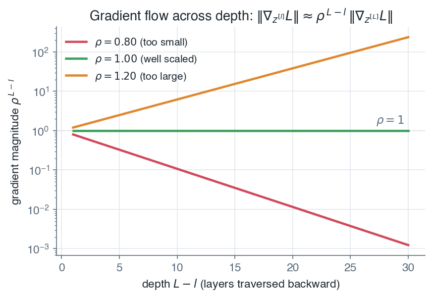
Gradient magnitude across depth: poorly scaled weights make it vanish or explode, while variance-preserving initialization keeps it near one.
Clip what still explodes. Initialization sets the scale once, at step zero. If gradients still blow up during training (frequent in recurrent networks, lesson 7), rescale the gradient so its norm never exceeds a threshold \(\tau\), keeping its direction:
\[\boxed{ g \leftarrow g \cdot \min\!\left(1, \frac{\tau}{\lVert g \rVert}\right) }\]4.2 Normalization
Initialization only positions the network at step zero: as training moves the weights, the distribution of every layer's input drifts, and later layers keep chasing a moving target. A normalization layer fixes the statistics on the fly: standardize, then let the network learn its scale back. For a feature \(x\) over a mini-batch of size \(m\), batch normalization computes
\[\boxed{ \mu_\mathcal{B} = \frac{1}{m}\sum_{i=1}^{m} x^{(i)}, \qquad \sigma_\mathcal{B}^2 = \frac{1}{m}\sum_{i=1}^{m}\left(x^{(i)} - \mu_\mathcal{B}\right)^2 }\] \[\boxed{ \hat{x}^{(i)} = \frac{x^{(i)} - \mu_\mathcal{B}}{\sqrt{\sigma_\mathcal{B}^2 + \epsilon}}, \qquad y^{(i)} = \gamma\, \hat{x}^{(i)} + \beta }\]The scale \(\gamma\) and shift \(\beta\) are learned like any weight, so normalization removes no capacity: the network can even learn to undo it. The payoff is a smoother loss surface, higher usable learning rates, and less sensitivity to initialization. Two practical consequences: at inference, where there is no batch, BatchNorm switches to running averages of \(\mu\) and \(\sigma^2\) accumulated during training (forgetting that switch is the classic BatchNorm bug), and the shift \(\beta\) makes the layer bias \(b^{[l]}\) redundant.
Layer normalization keeps the same standardize-scale-shift recipe but averages over the features of a single example instead of over the batch. Its statistics no longer depend on the batch, so it behaves identically in training and inference and handles variable-length sequences, which makes it the choice for recurrent networks and Transformers (lesson 10).
| Aspect | Batch normalization | Layer normalization |
|---|---|---|
| Normalization axis | across the batch, per feature | across the features, per example |
| Train vs inference | batch statistics vs running statistics | identical in both |
| Typical use | CNNs and feedforward vision models | RNNs and Transformers |
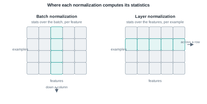
Batch normalization computes statistics down a feature column across the batch, layer normalization across the features of a single example.
4.3 Regularization and dropout
A deep network usually has more parameters than training examples, so it can memorize the training set, noise included. Regularization trades a little training accuracy for generalization, the bias-variance story of General concepts.
Weight decay (\(L_2\)). Add a penalty on the squared weights to the cost, with strength \(\lambda\):
\[\boxed{ J_{\text{reg}} = J + \frac{\lambda}{2}\sum_{l=1}^{L}\lVert W^{[l]} \rVert_F^2 \quad\Longrightarrow\quad W^{[l]} \leftarrow (1 - \alpha\lambda)\, W^{[l]} - \alpha\,\frac{\partial J}{\partial W^{[l]}} }\]The factor \((1 - \alpha\lambda)\) shrinks every weight at every step, hence the name. Its \(L_1\) cousin penalizes absolute values instead and drives many weights to exactly zero. Biases are left out of the penalty.
Dropout. On each training pass, keep every unit with probability \(p\) and zero it otherwise, then divide by \(p\) so the expected signal is unchanged:
\[\boxed{ \tilde{a}^{[l]} = \frac{m \odot a^{[l]}}{p}, \qquad m_i \sim \text{Bernoulli}(p) }\]No unit can rely on its neighbours, so the representation spreads out. Each step trains one of \(2^k\) thinned subnetworks that share their weights, and inference, with dropout off, approximates their average prediction for free (that is what the \(1/p\) buys). Typical keep probabilities: around \(0.8\) at the input, \(0.5\) in hidden layers.
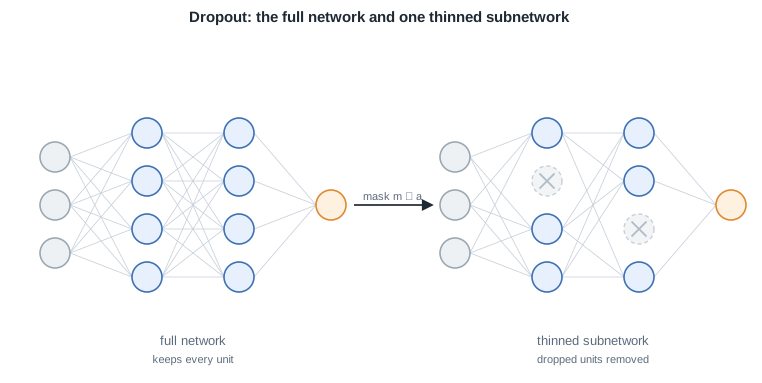
Dropout trains a different thinned subnetwork on each step by randomly removing units, and averages them at inference.
Initialized at the right scale, normalized in flight, and regularized against memorizing, the network is ready for architecture. The next lesson builds the convolutional network, whose weight sharing is itself a form of regularization.